Judging forecasts can be insanely hard than they are supposed to be. As time passes, the accuracy of a particular forecast seems obvious, but it is hardly so. The crux of the problem is the property that makes the forecasting different from classical predictions, i.e., time. The presence of temporal components makes it difficult to implement the techniques that we would have otherwise used, for instance, randomized control experiments. When it comes to time-series problems, only an omniscient being can replay a point in time multiple times to judge the effectiveness of the forecast. But unfortunately (or fortunately), we are no God, and unlike Dr. Strange, we got no Eye of Agamotto.
The evaluation is further convoluted when we express our forecasts in terms of probabilities. The issue here is not the nature of the problem but the way stakeholders perceive them. Probabilities are assumed by the readers as objective facts, not as likelihood estimates that they actually are. The biggest hindrance to this is that we humans have constructed an imaginary threshold in our heads, mostly at 50%, and we assume that the result, whichever side of this imaginary threshold it is falling on. Hence, the credibility of the forecasting model is erroneously judged by our limitations to comprehend probabilities. This fact is exemplified by the following scenario:-
Charaterstics of a good scoring system Link to heading
Particular forecasts can’t be judged but if a model predicts forecast tomorrow, and the day after tomorrow and the day after, and so on, these results can be tabulated and the track record can be determined. If the forecasting model is perfect, the rain will happen 70% of the time when the model predicts a 70% chance of rain. This process of measuring the accuracy of probabilistic forecasts is called calibration and can be illustrated with the graph below:-
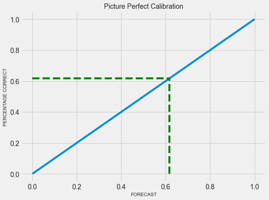
Fig 01 - Perfect Calibration
A diagonal line (x = y) implies perfect calibration. But there would be cases where the model makes conservative forecasts. For instance, the model predicts a 45% likelihood of rain when the actual probability is 60%. In this case, the calibration curve would be far over the diagonal line. Similarly, the calibration curve would be far under the diagonal line when the model makes very optimistic forecasts, that is, predicting things are 80% likely when the chance of occurring is around 50%.
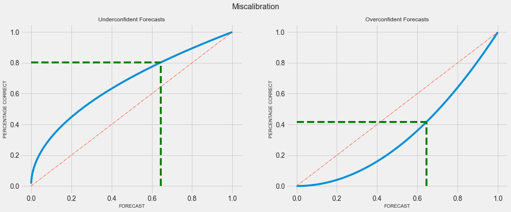
Fig 02 - Miscalibration
Calibration can be used to improve the models where the results show that it has mistakes with the high probabilities. It can be of great use in cases where the exact value of the probability is taken into account while making decisions. There are a couple of caveats with this method though:-
- It only works for the cases where the events stack up fast. So, it works better for daily weather forecasts, predicting whether users will click or not, etc. It will not work for things like GDP forecasts because it will take a quarter to half a century for results to pile up.
- As we require a high number of forecasts for this method, it becomes increasingly difficult to judge “rare” events forecasts.
Note:- One doubt that generally surfaces here is how the calibration is different from ROC-AUC curve? While both metrics take prediction scores as input, ROC-AUC only focuses on ranking predictions. Many mistakes these probabilities as a prediction as probabilities and stop evaluating their model beyond measure of accuracy.
While Calibration is important, we do require another measure to express the degree to which one can sort correct and incorrect items into different buckets. This can be referred to as Resolution, and mathematically can be expressed as the degree to which predicted probabilities placed into subset differ in true outcomes to the average true outcome. Calibration and Resolution are the contrastive representations of probability judgments. The former is a designated form that presupposes a particular coding of outcomes (e.g. click vs no click or rain vs no rain) and the latter is an inclusive form that incorporates all events and their complements. So, the probabilistic forecasts can be evaluated by the following criteria:-
- Calibration:- expressed as correspondence between the subjective and objective probabilities.
- Resolution:- expressed as the ability to distinguish between events that do and do not occur.
When we combine Calibration and Resolution, we get a scoring system that can capture exactly what good forecasting should do.
Brier Score Link to heading
Taking the above measures into consideration, Brier Score, a metric used in binary classification problems, qualifies as a proper scoring rule. It minimizes the squared between the predicted probability of a label and its true label. Brier Score is a single number composed of three measures, reliability, uncertainty, and resolution. The reliability can be defined as the overall measure of calibration that quantifies how close predicted probabilities are to the true likelihood. Uncertainty and resolution, when combined can also be aggregated into the measure called “refinement” which is associated with the area under the ROC curve, and when added with reliability, yields Brier Score. Hence, in layman terms, Brier Score can be defined as:- $$ BS = Reliability - Uncertainty + Resolution $$
Mathematically, the Brier Score can be defined as:- $$ BS = \frac{1}{n}\Sigma_{i=1}^n(p_{i} - o_{i})^2 $$
where:
- $n$ is the number of events under consideration
- $i$ indexes the events from 1 to $i$
- $p_{i}$ is the forecast probability for the $i^{th}$ event
- $o_{i}$ is the outcome of the $o^{th}$ event
As it is the distance in the probability domain, the lower the score the better and a perfect forecast would yield a Brier score of 0. The forecast that is wrong to the greatest extent (i.e. 100% wrong) will fetch a score of 1 and a random guess would earn a Brier score of 0.5. Brier score can be used when we want to:-
- Measure model’s confidence in its predictions
- Calculate probability estimates
- Calculate error distribution
This makes Brier Score super-useful in high-risk applications.
Though Brier Score is a single number, it can be decomposed into three components, which captures different dimensions of a forecast. This might be due to the fact that the Brier Score is made out of other forecasting metrics.