Depending upon the nature of the problem and the functioning of the model, the format in which output is provided can differ from model to model. For instance, in a multiclass classification problem, a decision tree provides a label, which is narrowed down going down the tree, where each node reduces the set of possible outcomes to one. On the contrary, the neural networks provide a vector of continuous values calculated by applying non-linear transformations to the input vector. In the latter case, we have to transform the output vector to a single label (here, looking at you, argmax). Here, there might be a temptation to use these values as the confidence of the model in each label class. After all, isn’t the model that has twice the confidence in the label class for which output is 0.6 to the label class for which the output is 0.3? NO. Not until the model is calibrated.
Calibration is a post-processing technique used to improve the probability estimate of an already trained model, in order to improve its performance. For instance, among the samples that have a 0.8 probability of belonging to a particular class, we want at least 80% of them to be true. A model is perfectly calibrated if, for any p, a prediction of a class with confidence p is correct 100*p times out of 100.
$$ P(\widehat{Y} = Y | \widehat{P} = p) = p, \forall p \in [0,1] $$ where,
- $\widehat{Y}$ is the predicted label
- $Y$ is the actual label
- $\widehat{P}$ is the predicted probability estimation
- $p$ is the actual probability
Though calibration seems like a simple technique, miscalibrated models are actually the norm. Some models are miscalibrated out-of-the-box. For instance, Gaussian Naive Bayes pushes the output response closer to 0 or 1 because it assumes feature independence. On the other hand, results in Random Forest are very rarely approaching (or equal to) 0 or 1, because the output responses in Random Forest are average of the outputs of numerous underlying decision trees. No doubt, one can get predictions equal to 0 or 1 in the case of Random Forest, but that is quite rare from a probabilistic point of view. Neural Networks are even more prone to miscalibration, given the high number of hyperparameters being used. The depth and width, regularization (weight decay), and batch normalization can all contribute to miscalibration. Given so many variables can contribute to miscalibration, it is safe to never assume that the model is calibrated.
Is my model miscalibrated? Link to heading
Now that we know calibration is a thing, how do we know whether our model requires calibration or not? For that, we can use calibration plots. They are the most common ways to check whether the model is miscalibrated or not. Calibration plots are often line plots, where on the y-axis, the proportion of true probabilities, and on the x-axis, the predicted probability is plotted. But these probabilities are not plotted as such. They need to be first binned by the probability estimation that the model made. For instance, we can take all the predictions in the range of 0 to 0.2 and put them in the same bin and predictions between 0.21 and 0.4 in the other, and so on. Then, for each bin, the percentage of positive samples is calculated.
Example Link to heading
For the sake of this example, I will be using Breast Cancer Dataset. This data is readily available in Scikit Learn Dataset API and can be imported as follow:-
import pandas as pd
from sklearn.datasets import load_breast_cancer

bcd = load_breast_cancer()
df = pd.DataFrame(
    data=bcd.data,
    columns=bcd.feature_names
)
df["target"] = bcd.target
The label is a binary variable, 0 and 1, where 0 stood for benign and 1 for malignant tumor. The aim here is to train a simple Random Forest Classifier and plot the corresponding calibration curve. For simplification, I am doing a random train-test split and “fitting” an RF Classifier. As we require probabilistic predictions for plotting the calibration curves, we are calling the predict_proba method on the trained model object.
from sklearn.ensemble import RandomForestClassifier

feature_df = df.drop(columns=["target"])
target_df = df["target"]

x_train, x_test, y_train, y_test = train_test_split(
    feature_df,
    target_df,
    test_size=0.2,
    random_state=19
)

RF = RandomForestClassifier(random_state=19)
rf_classifier = RF.fit(x_train, y_train)
rf_preds = rf_classifier.predict_proba(x_test)
Once the class probabilities are captured, the next step would be to compute the bins for the calibration plot. One can use Scikit-learn’s calibration_curve method to compute the true and predicted probabilities for a calibration curve. This method, discretize the probability range of [0, 1] into a number of bins, mentioned in parameter n_bins, passed in the method above. Here, we are creating 10 bins:-
cal_y, cal_x = calibration_curve(y_test, rf_preds[:, 1], n_bins=10)
After this, we can plot a simple line plot using Seaborn.
import matplotlib.pyplot as plt
import seaborn as sns
plt.style.use("fivethirtyeight")

sns.lineplot(x = cal_x, y = cal_y, markers="*", label="Random Forest")
plt.xlabel("FORECAST", fontsize = 10)
plt.ylabel("PERCENTAGE CORRECT", fontsize = 10)
plt.title("Calibration Plot for Breast Cancer Data", fontsize = 14)
plt.legend()
plt.show()
Calibration plot:-
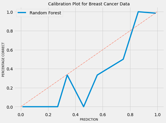
Fig 02 - Miscalibration
The calibration of the model is way-off, but we can see horizontal lines from 0 to 0.25 and from 0.85 to 1. This means that model is pushing predictions closer to 0 and 1 in their respective neighbourhood. This implies that the model is discriminative. We can also look explore how many predictions, the model has made, in each bin.
def bin_total(y_true, y_prob, n_bins):
    bins = np.linspace(0, 1, n_bins + 1)
    binids = np.digitize(y_prob, bins) - 1
    return np.bincount(binids, minlength=len(bins))
bin_total(y_test, rf_preds[:,1], n_bins=10)
>> array([32,  2,  1,  3,  2,  6,  0,  2,  1, 29, 36], dtype=int64)
As we can see from the above result, most of the predictions are either near 0 or 1. Very few are in the maybe category. So, the above model is a good discriminator, but poorly calibrated.
Why is binning required? Link to heading
As in the equation above, the probability can’t be computed using a finite number of samples, since $\widehat{P}$ is a continuous random variable. Therefore, to empirically measure the model’s calibration, several statistics techniques are designed and binning is one such technique. By binning samples, we can calculate expected sample accuracy as a function of confidence, while reducing the effects of minor observation errors. It is required for bins to have equal width to ensure plot readability.
Point Estimates of Calibration Link to heading
While Calibration Plots are a reliable visual tools, it is equally important to have a scaler summary statistics for calibration. We discuss two of such methods.
1. Expected Calibration Error Link to heading
Expected Calibration Error (ECE) measures the difference in expected accuracy and expected confidence. Mathematically, $$ \mathbb{E}_{\widehat{P}}[|\mathbb{P}(\widehat{Y} = Y | \widehat{P} = p) - p|] $$
In practise, ECE can be calculated by partitioning the predictions into M equally-spaced bins (as we did in Calibration Plots) and taking a weighted average of bins’ accuracy and confidence difference. This can be denoted as:- $$ ECE = \sum_{m=1}^{M} \frac{|B_m|}{n} |acc(B_m) - conf(B_m)| $$
Here, $n$ is total number of bins. For perfect calibration, ECE should be $0$. Hence, $acc(B_m)$ should be equal to $conf(B_m)$.
2. Maximum Calibration Error Link to heading
Maximum Calibration Error (MCE) is preferred in the high-risk application where reliable confidence measures are absolutely necessary. Empirically, MCE can be defined as follow:- $$ MCE = max_{m \in [1 … M]} |acc(B_m) - conf(B_m)| $$
Conclusion Link to heading
In this post, we tried to establish what is the intuition behind the Calibration, why it is important and how can we measure it. In the continuation of this post, we will ponder over the techniques that can effectively remedy the miscalibration.